Notes on Platform Architecture
The Araudia platform consists of ~15k lines of code organised into four main parts:
engine/Stochastic simulation engineode/ODE checker for individual simulation segmentsanalysis/General data analysis tools (applicable to all simulations)unit/Unit tests
Additional scripts were added to produce the results in Our Paper:
rstb/Specific data analysis tools, and a HPC Loader script to send groups of simulations to an SLURM-based HPC computing cluster.
Simulation Engine Main Loop
The Araudia codebase is built on the core assumption that ecological and evolutionary processes operate at clearly separated time scales. Hence, a simulation executes using an outer loop (handling slower evolutionary events) which repeatedly calls an optimised inner loop (handling faster metabolic and ecological population dynamics events).
The outer loop is not time-critical, and runs as normal Python code. It handles infrequent structural changes to the dynamical system, i.e. events such as new protocell type creation, protocell type extinction, and changes in the reactor feed concentrations. The inner loop is time-critical and executes as machine code (Python JIT compiled by NUMBA). It runs the Gillespie algorithm to simulate frequent micro-events in a protocell ecology, such as chemical particle movements and normal protocell division events.
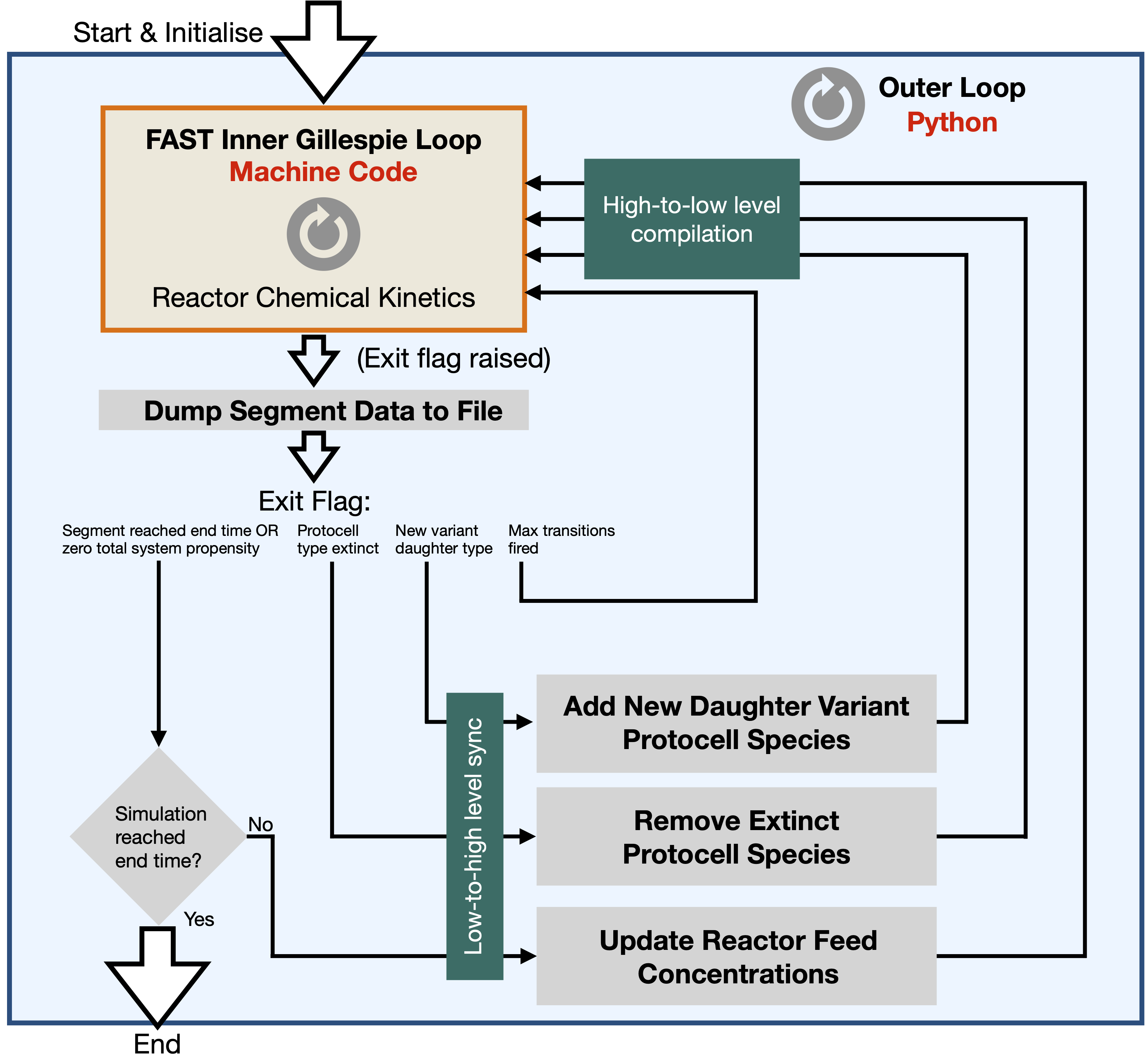
The module reactor.py ‘glues’ all components of the platform together and executes the logic below:
Initialisation. The simulation is initialised as a series of high-level Python objects, plus other settings. In particular, a list of configured
ProtocellTypeobjects is specified, with each object containing an initialisedMetabolicNetwork,RegulatoryNetworkandResourcePoolobject.High-level to low-level compilation. The high-level objects and other settings are “compiled” by
transitionsystem.pydown to low-level numeric numpy arrays (containing state variables, parameters and transition information) for Gillespie simulation by optimised scriptssa.py. Critically, thetransitionsystem.pymodule automatically builds a dependency graph of events within the system, such thatssa.pycan selectively update entries in the system propensity vector when a particular event is fired. For a large system of events, this represents a huge efficiency saving with respect to updating the whole propensity vector every time an event is fired. (Theplot()andeff_plot()methods intransitionsystem.pyshow the event dependency graph and a barchart showing selective update efficiency savings, respectively).Inner Gillespie loop. The next “segment” of the simulation is executed by
ssa.py. A “segment” is a window of time over which there is a constant protocell ecology: there are no births of new protocell types nor extinctions of existing protocell types, and the reactor feed concentrations do not change. The inner loop exits when one of the following five conditions occurs:The end time of the segment is reached (because the feed concentrations are about to change, or the simulation has ended)
The number of transitions fired have reached an upper limit number (around 5 million)
The system has zero propensity (no further viable events exist in this segment)
A new protocell type is created
A protocell type has become extinct
The state vector of the simulation and all current parameters are dumped to a pickled file with
.infoextension, for the segment.Low-level to high-level synchronisation. Changes in the system state that took place during the segment (e.g. chemical levels or protocell population levels in the reactor) are propagated back up to the high-level Python objects.
Outer loop. Changes are made to the structure of the dynamical system. The
TransitionSystemis told to update feed concentrations, to delete protocell types with zero copy number (decreasing state vector size), or to add a new daughter variant protocell type in a single copy (increasing state vector size). New daughter variants are produced by theProtocellTypeclass, using standard Python code.If the end time has not been reached, execution continues from Step 2 above.
Therefore, rather than having monolithic execution from beginning to end, the simulation runs as a consecutive series of independent “segments”. This has several important advantages:
Memory requirements are kept manageable, as data is dumped to file after each segment finishes. Each segment can fire a maximum of 5 million events.
Segments give a natural way to reduce detailed simulation trajectory information down to more manageable data sizes. System state is normally only recorded at the beginning and end of each segment, and not in-between.
The simulation can be
ctrl-cforce-quit at any stage, without loss of all simulation data to that point (only loss of the current segment).
Using standard Python code for the outer loop is convenient because high-level classes can handle complicated events such as producing a variant daughter protocell type. High-level classes are easy to read, debug and unit test (see unit/ directory).
An ODE checker (odecheck.py) was built to verify the stochastic solver in each simulation segment, where the boundary conditions of the dynamical system are fixed. The ODE checker gives dynamical behaviour in the large system size limit, but it is still a useful indicator that the optimised stochastic simulation code is implemented correctly. The ODE checker implementation is completely independent of the stochastic engine: it just initialises itself on .info files output by the stochastic engine.
The simulation analysis scripts (in analysis/) are also implemented independently of the main engine code. They simply read .info files in an output directory to display a series of graphs. The analysis scripts are generally applicable to any simulation. More specialist analysis scripts can be written for particular simulations (as is done in the rstb/ directory).
Neural ODE Implementation
The regulatory network of a protocell is implemented as a neural network which controls the propensity of internal enzyme level changes. Firstly, a non-optimised version of the neural network calc was created in the calculate_enzyme_level_derivatives() function of the engine/regulatorynetwork.py class, using numpy matrix multiplication operations. Then, an optimised version for numba was created as the calculate_enzyme_level_derivatives() function of the ssa.py module. These two implementations were tested as being numerically identical. The simulation itself only uses the optimised version in ssa.py.
The optimised version in ssa.py assumes that all enzyme costs are 1.0, such that the total enzyme cost can be calculated quickly as a simple sum, rather than as a weighted sum. This hard-coded requirement for enzyme costs to be 1.0 is stated when the platform initialises.
Main Groups of Scripts
Core simulator:
engine/ssa.py(uses numba JIT compilation)engine/transitionsystem.pyengine/reactor.pyode/odecheck.py
High-level classes to initialise and modify properties of protocell types:
engine/protocelltype.pyengine/metabolicnetwork.pyengine/resourcepool.pyengine/regulatorynetwork.py
Other satellite scripts:
engine/iohandler.pyengine/chemicaluniverse.pyengine/initialecologies.pyengine/constants.pyengine/feedschedule.pyengine/parametercheck.py
Data analysis scripts (general):
analysis/analysis.pyanalysis/analysisL.py