Illustrative Demos

Araudia can be used to investigate a plethora of different (proto)cell evolution scenarios, from controlled scenarios to more exploratory unconstrained simulations. Multiple options exist: evolution can be enabled, internal regulatory capacities can be enabled, the initial condition can be set to any ecology and the chemostat can have any type of time-dependent nutrient inputs applied.

The demos on this page just give a quick illustration of some capabilities using small protocell ecologies. The Paper Case Studies section at the end gives the simulation files to reproduce the the three case studies reported in Our Paper.

For more detail on the various options available for simulation and analysis, see the Simulation Settings and Analysis Settings pages.

Preliminary Notes

The results you obtain may differ from some of the demo results shown below. Simulation trajectories are sensitive to initial conditions, the chance application of evolutionary events, and to stochastic fluctuations.
A small “burn-in” time is always required for the initial ecology to equilibrate to steady state inside the reactor (10000 time steps is more than enough). Then, the simulation can be considered active.
On a modern computer, and for default parameters, it can take up to 1 minute (wall clock time) to simulate 3500 arbitrary time units when regulation is enabled. Hence, a simulation of 5 million time units can take up to 24 hours to complete. Simulations are faster when regulation is disabled because neural network calculations are not necessary.
Simulations do not need to run all the way to the end time. They can be stopped prematurely at any time by typing ctrl-C. Then, analysis can be performed in the standard way.

Before running the demos below, first change to the demo/ directory:

cd protocell
source venv/bin/activate
cd araudia
cd demo

Demo 1: Chemical Pulses Running Through Chemostat

This demo simulates 5 different nutrient chemicals being applied to the chemostat in pulses. No protocells exist in the chemostat in this simulation, only chemicals. The first command below runs the simulation, and the second runs the data analysis:

python3 r1.py
python3 a1.py

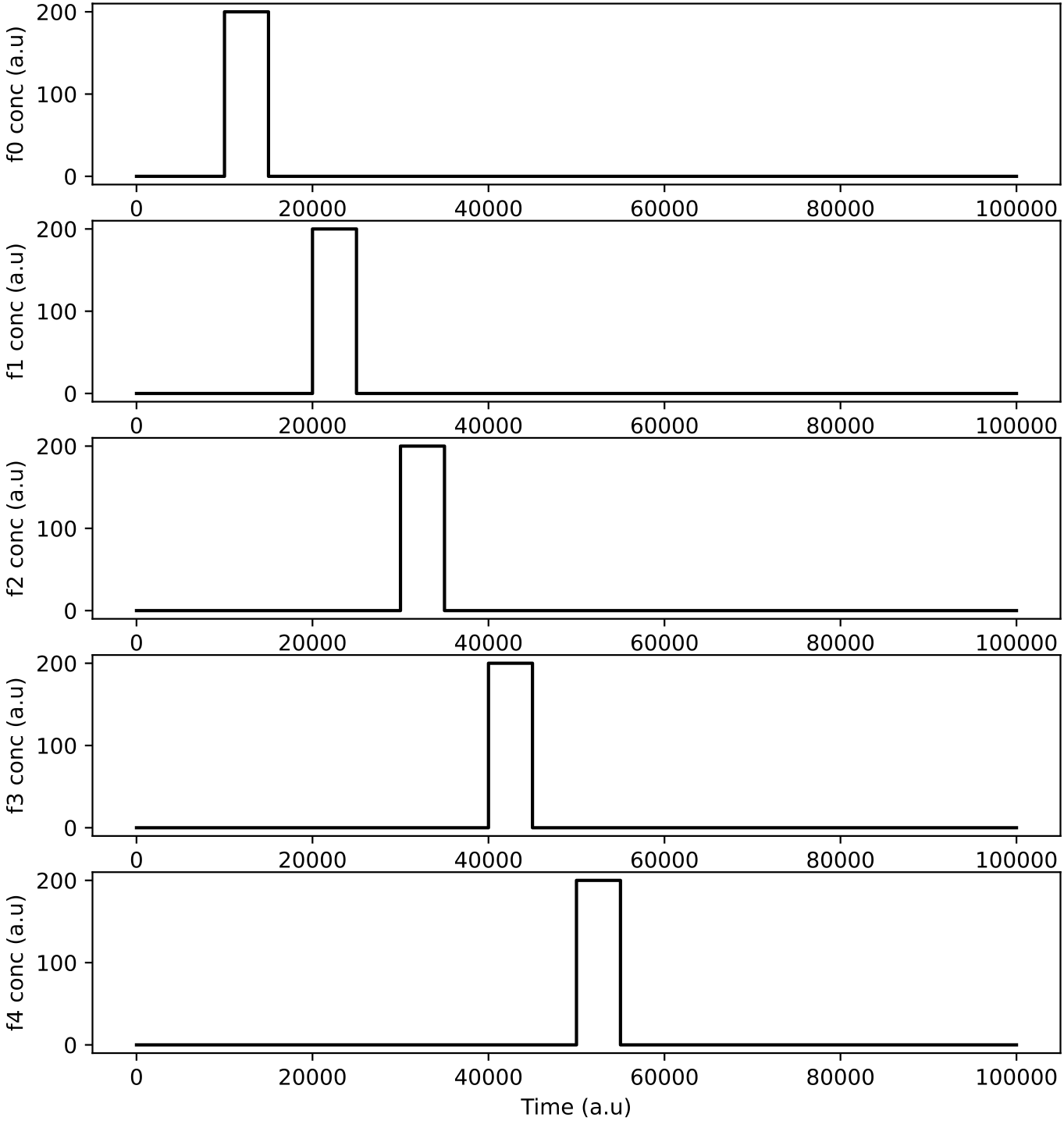
Araudia will first display the reactor feeds (left, above), and will start the simulation if they are confirmed as correct.

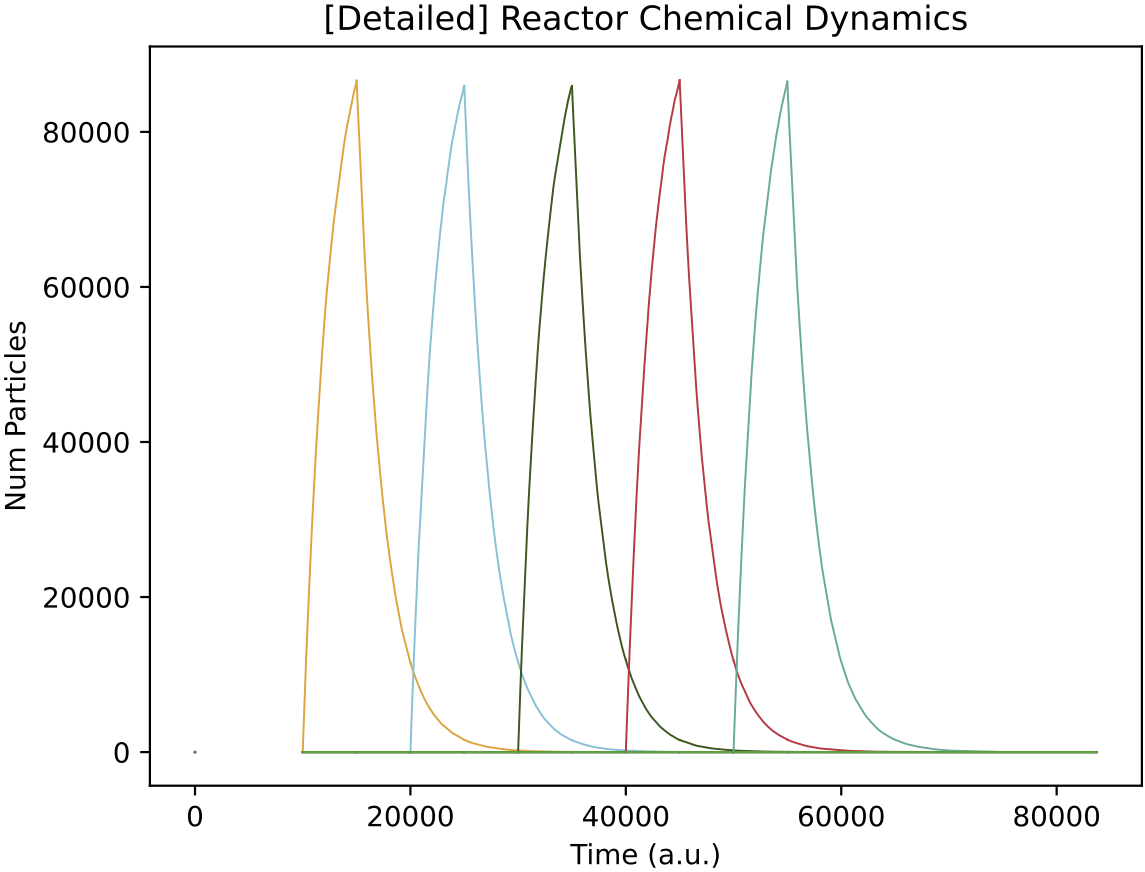
The peaks of chemical concentration inside the chemostat (right, above) take time to rise and overlap, due to the relatively slow chemostat dilution rate (set to "MU": 0.0004 in r1.py). You can experiment with different dilution rates, and/or chemostat volumes ("OMEGA" setting in r1.py). Faster dilution rates and larger volumes take more time to simulate as there are more particle movement events.

Demo 2: Single Population Sustaining in Chemostat

Here, the chemostat has a constant single nutrient source applied and a single protocell type at 100 copies exists initially. Evolution is disabled, and the protocells don’t have the potential to develop regulatory networks. The population sustains inside the chemostat, i.e. its growth rate balances the dilution rate of the reactor:

python3 r2.py
python3 a2.py

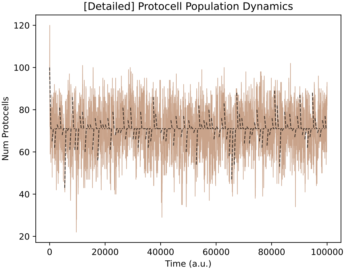
Demo 2: Protocell population sustaining at 60 copies

In this particular run, the protocell population sustains with a mean of 70 copies in the chemostat.

However, the import enzyme level in the protocell type is initialised randomly. In some simulations, the import enzyme level will be too low and the protocell population will become extinct after a short time.

The black dotted lines on the above plot show the behaviour predicted by the deterministic ODE equations in each simulation segment (because option "ODE check" : True is set in a2.py). There is good agreement, both in the initial behaviour, and with the mean population size predicted by the stochastic model.

Demo 3: Single Population under Evolution (Major Innovations Enabled)

Returning to the population of a single protocell type, this example follows what happens over a longer time period, when evolution is enabled (note: regulation is still disabled). Two constant nutrient feeds are supplied to the chemostat, but the protocell type initially feeds from only one of them. Major innovations can happen in evolution, and so the protocell type can potentially evolve to import and grow from the second nutrient source also:

python3 r3.py
python3 a3.py

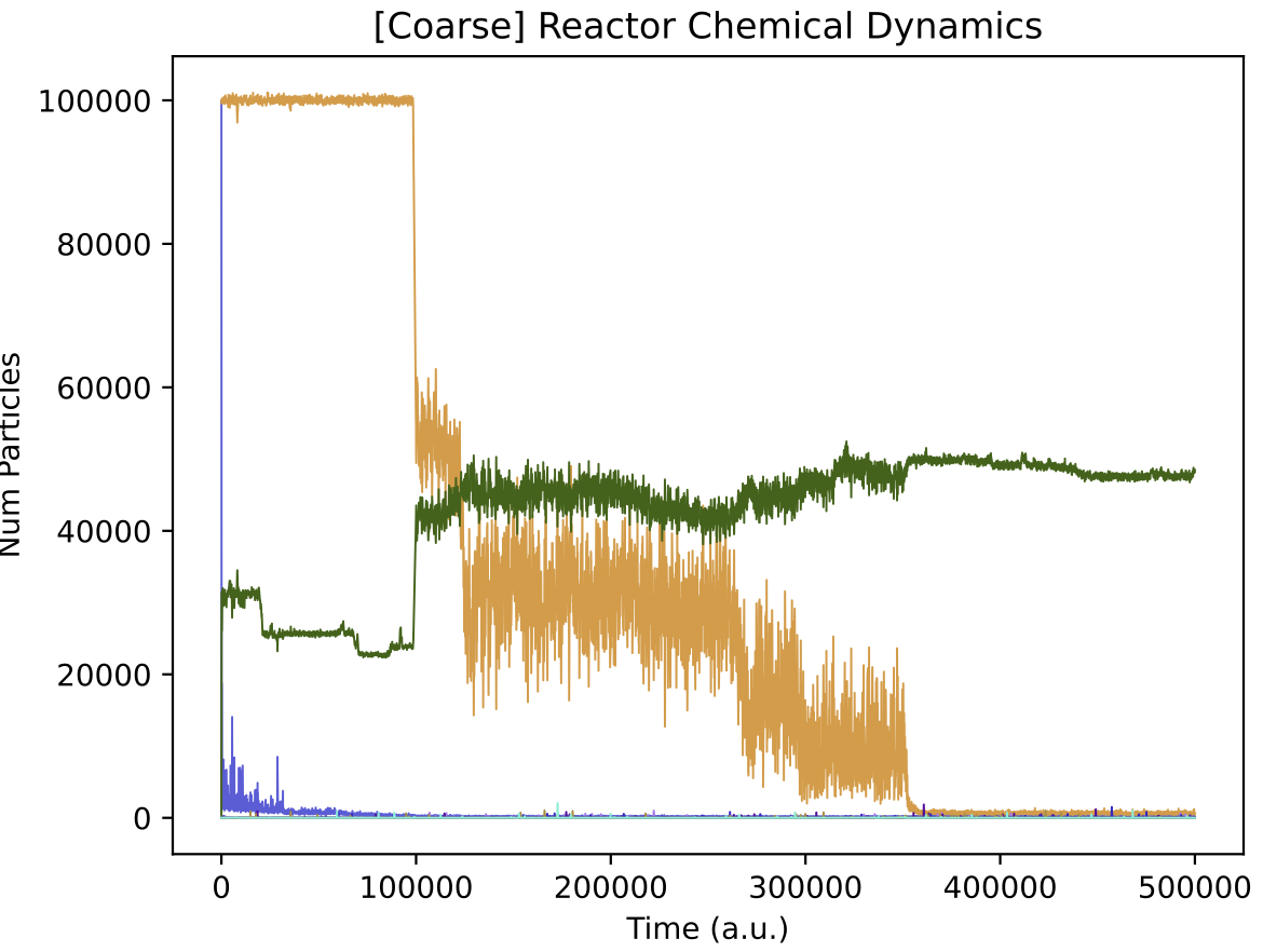
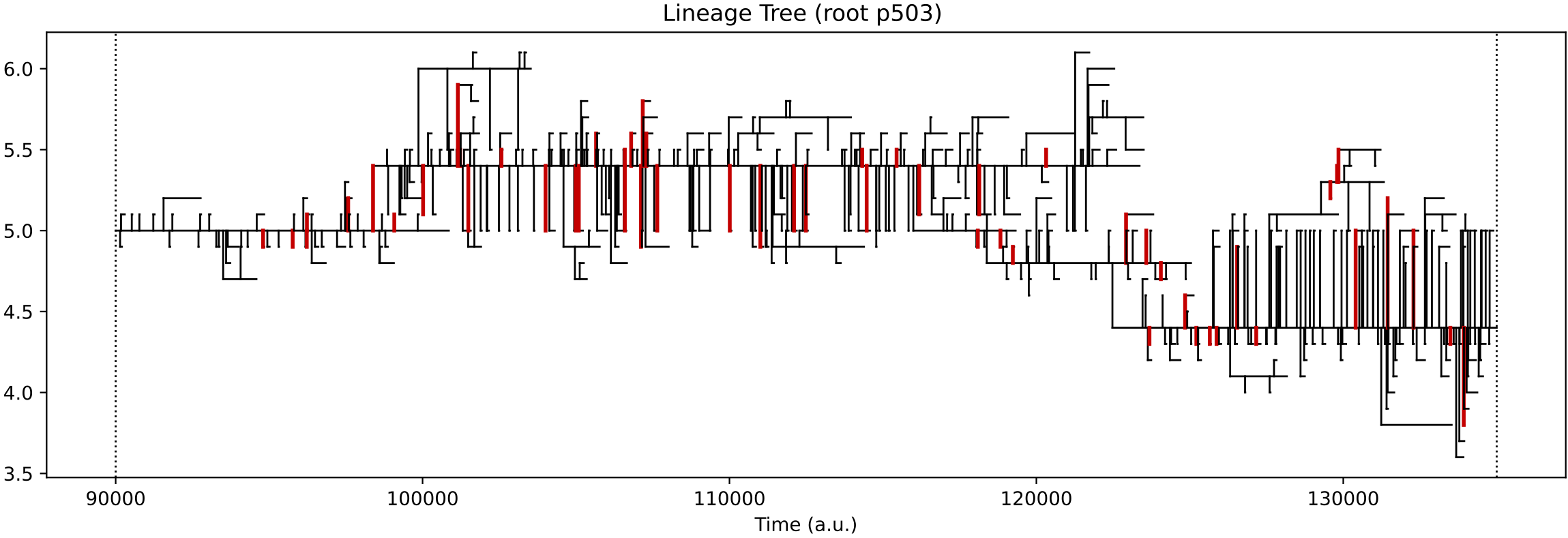
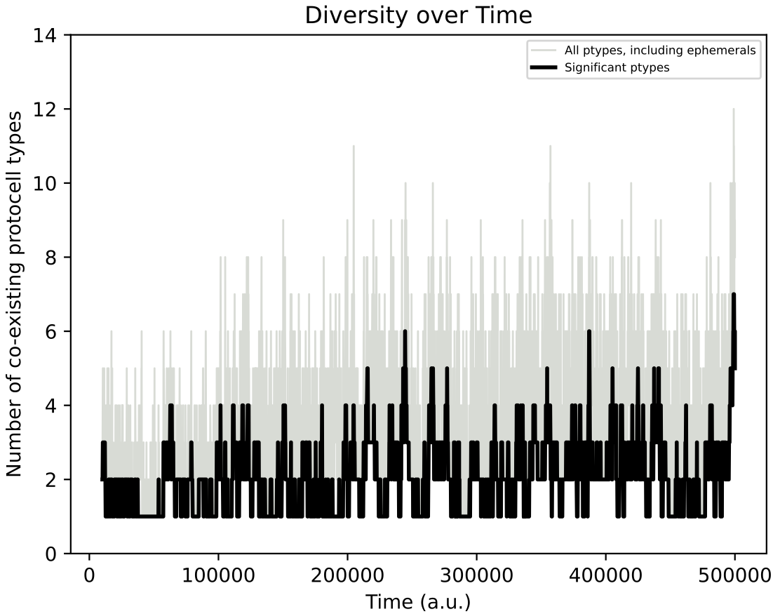
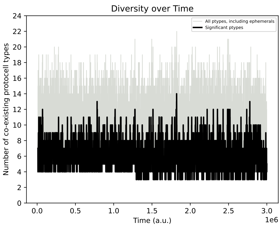
In the simulation above, at around 100k time steps, a major evolutionary innovation occurs whereby the protocell type begins feeding on both nutrient sources. This is evident by the population size increasing (top left) and by the chemostat chemical dynamics qualitatively changing (top right). The evolutionary lineage plot produced (middle) shows that a major innovation (red vertical bar) establishes a new stable lineage at around 100k time steps. The ‘diversity over time’ plot created shows that normally around 2 protocell type “quasispecies” co-exist, but this number can increase to as many as 10 quasispecies (this plot corresponds to vertical slices through the lineage plot).

It is interesting to investigate what very long term effects of evolution might be in this case. For example, given correct conditions, could a stable cross-feeding ecology eventually emerge, containing individuals with different diets that excrete different waste products?

Demo 4: Single Population Evolving Lac-Operon-Like Behaviour

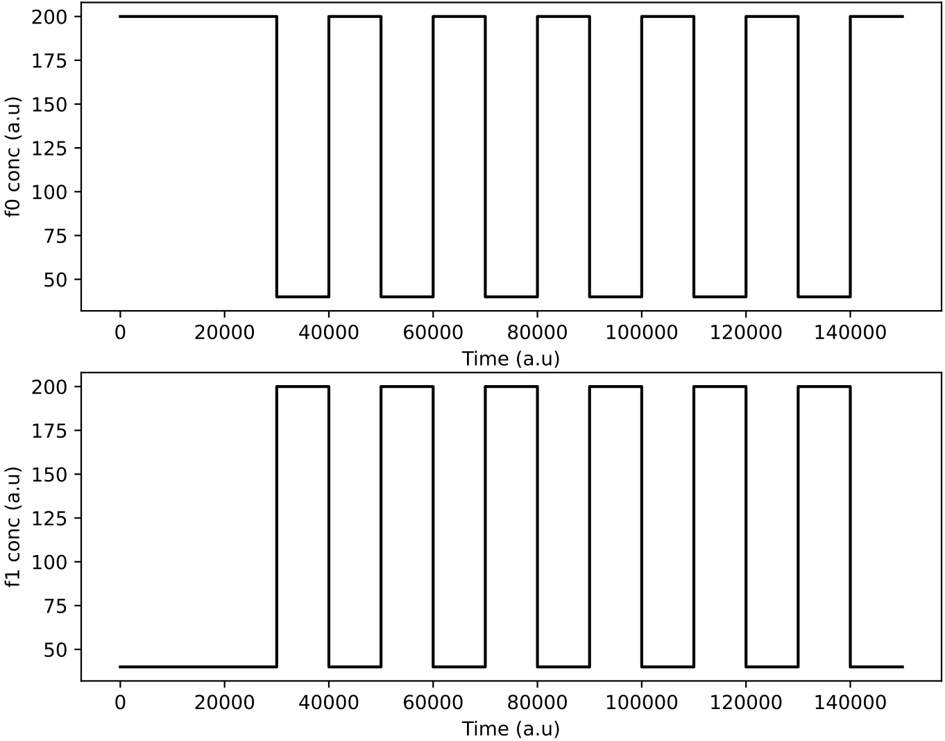
In this demo, the initial population of protocells is a single type that feeds from both nutrient sources. The nutrient inputs to the chemostat are varied as short period square waves, 180 degrees out of phase – when nutrient chemical 0 is present at a high value, then nutrient chemical 1 is at a low value, and vice versa.

Regulation is now turned on and so protocells have the potential to evolve dynamic control of nutrient preference. The aim is to ‘learn’ to up-regulate the enzyme corresponding to the most abundant nutrient in the environment, and down-regulate the other enzyme (as e.g. E.coli do when glucose becomes absent but lactose is present).

Evolution introduces minor mutants, but major innovations are turned off (have 0 probability). Hence, protocells always ‘eat’ nutrients 0 and 1 in this example; they cannot change their diet.

python3 r4.py
python3 a4.py

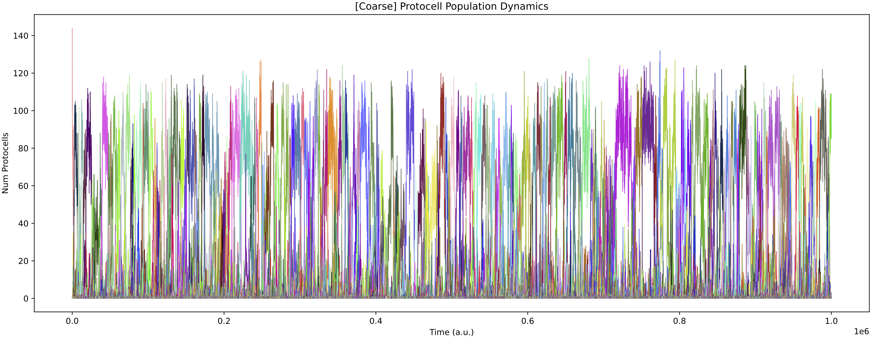
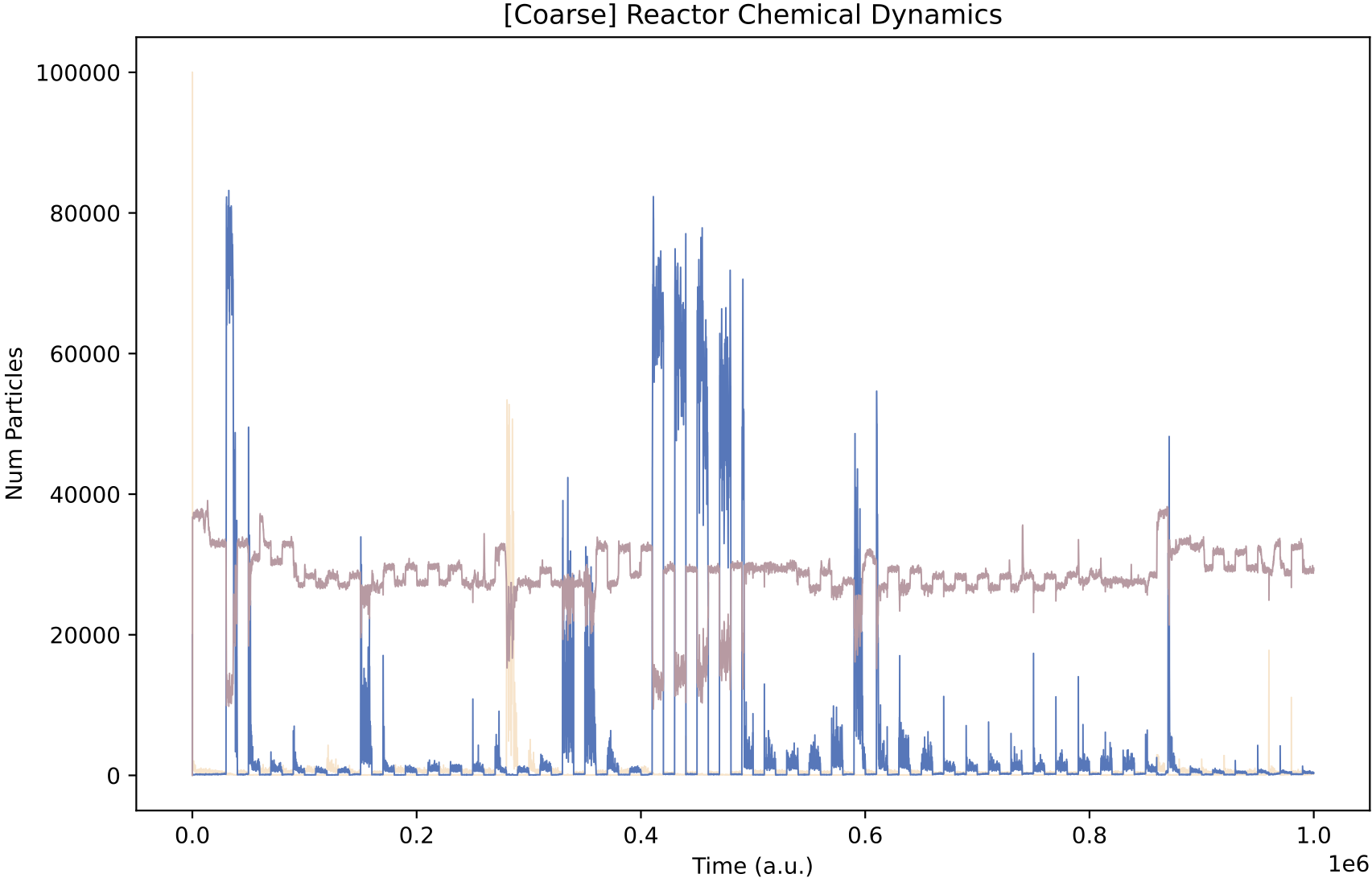
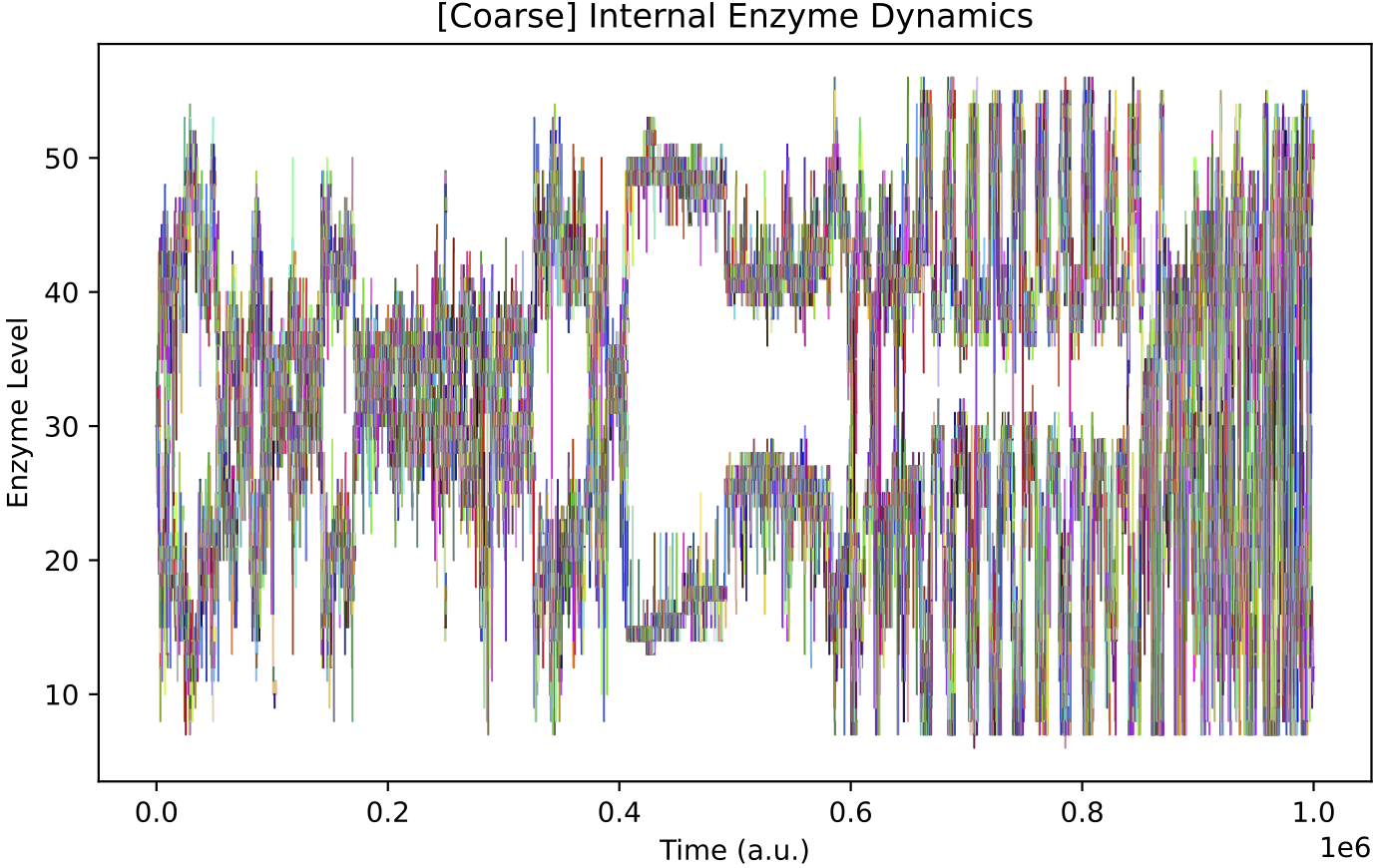
This simulation presents a case where a more specialist analysis of the internal enzyme dynamics is required. The general enzyme dynamics plot above contains the internal enzyme levels of all protocell variants and the sheer amount of information obscures important details.

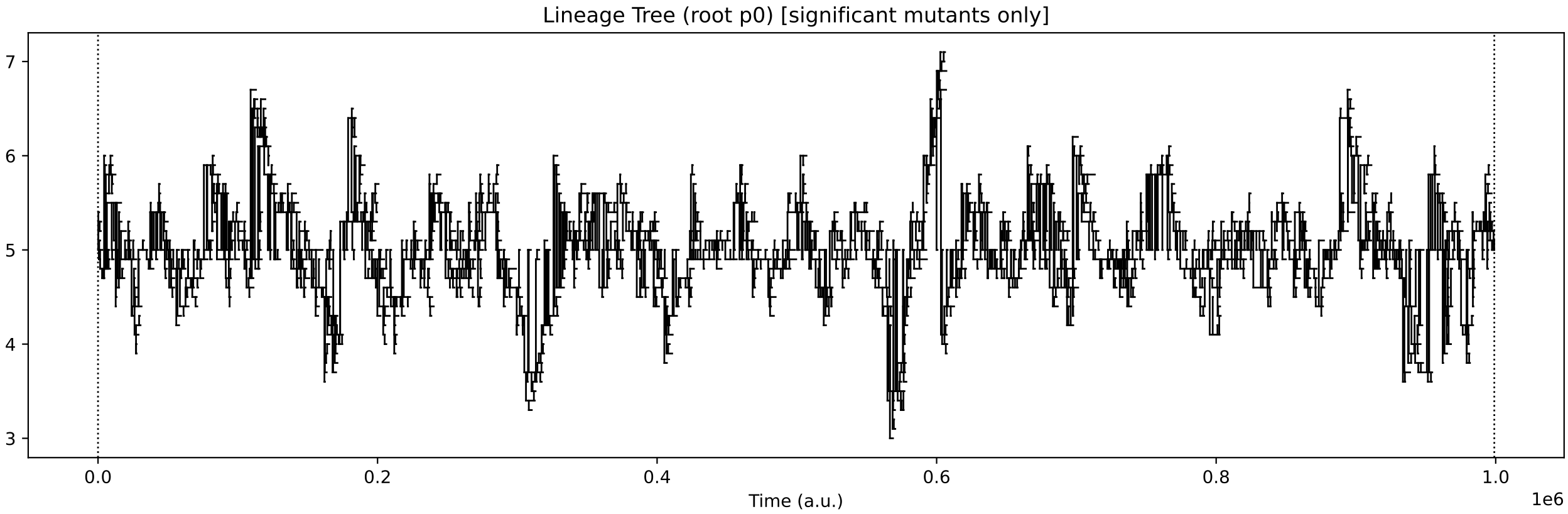
It is more instructive to just follow enzyme dynamics across the species which form the “trunk” of the evolutionary lineage. This demo is similar to Case Study B1 in Our Paper. As such, we can use code in the B1 analysis tools to better track enzyme levels just across the “trunk” species:

cd ..
cd rstb
python3 analysisB1.py

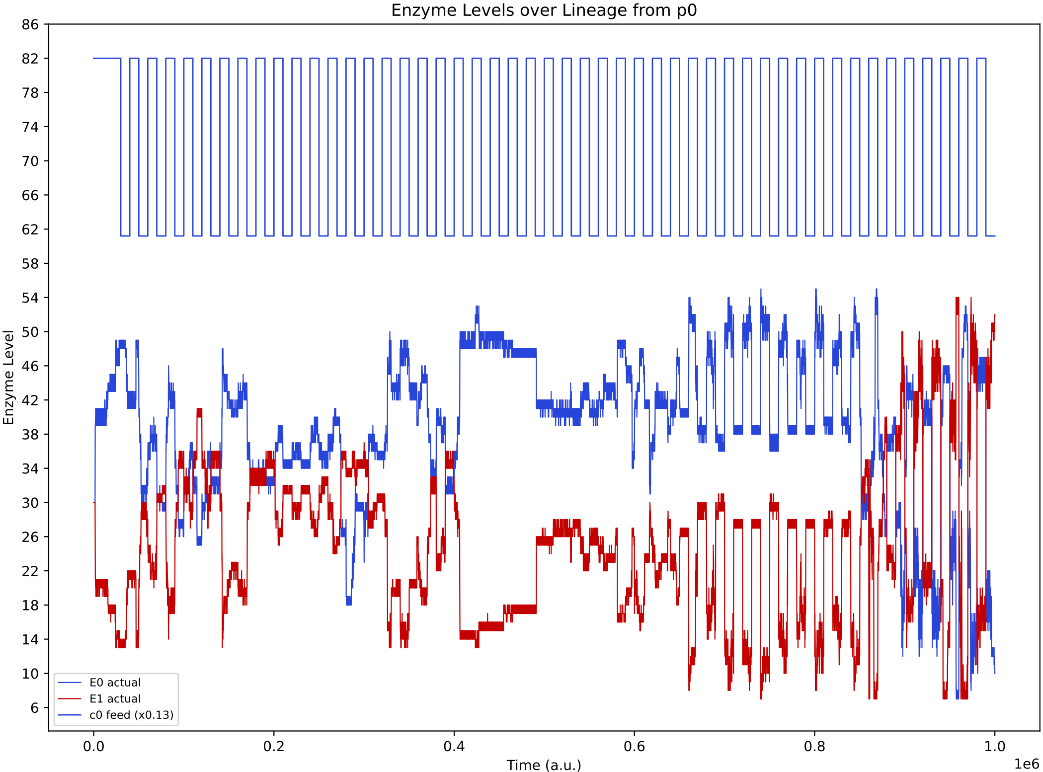
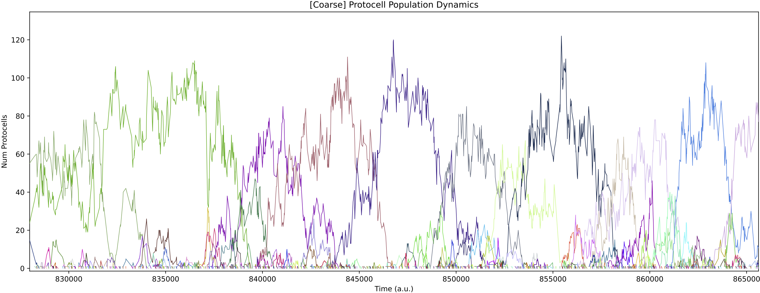
Demo 4: Enzyme dynamics in main trunk lineage

Now, it is more obvious that regulation emerges at around 850k time steps. From this time, the E0 and E1 internal enzyme levels have large fluctuations in synchronisation with the chemostat nutrient forcing, allowing the single species of protocell to grow maximally from the provided nutrients.

This demo highlights that general analysis tools supplied with Araudia sometimes need to be extended in order to capture important phenomena (particularly in complex evolutionary simulations that involve major innovations).

Demo 5: Testing an Evolved Regulatory Network

At 965k time units in Demo 4 above, the main lineage protocell type in the reactor (p19055) is displaying internal enzyme switching behaviour.

To verify that this behaviour is caused by the regulatory network, and not just be phylogenetic adaptation, we can run a simulation just containing that protocell type (at 100 copies initially), and turn evolution off:

python3 r5.py
python3 a5.py

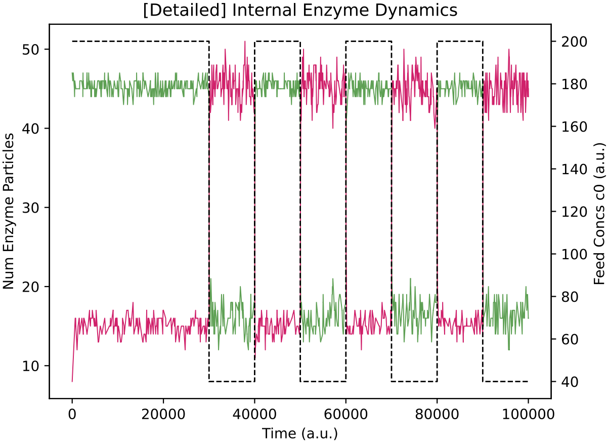
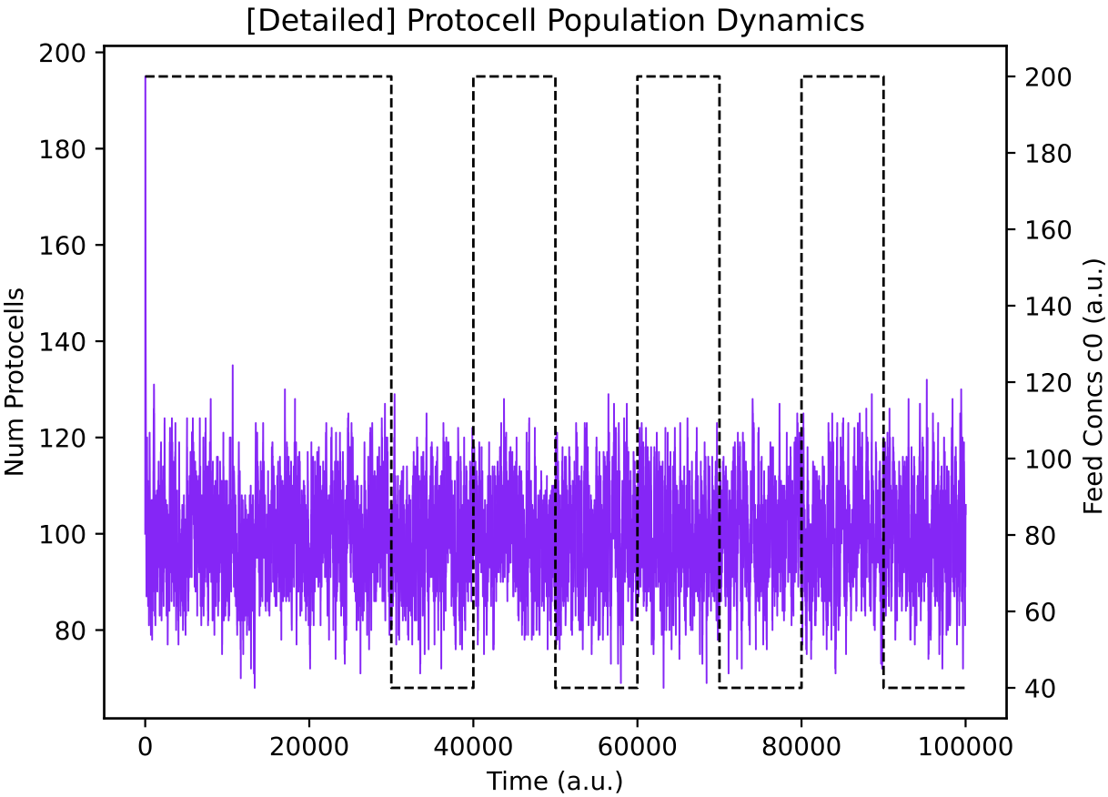
This protocell type, p19055, is indeed switching internal enzyme levels (E0 = green, E1 = red) using its regulatory network (left) and it maintains a stable population size (right) in the face of alternating nutrient supply. The black dotted line in plots above shows the concentration of chemostat feed 0, and is plotted on the second y-axis. Chemostat feed 1 varies high and low in the opposite sense to feed 0, and is not plotted for clarity.

In contrast, at 450k time units in Demo 4 above, the main lineage protocell type in the reactor (p8790) is not switching internal enzyme levels in response to nutrient levels. This can also be verified:

python3 r5a.py
python3 a5.py

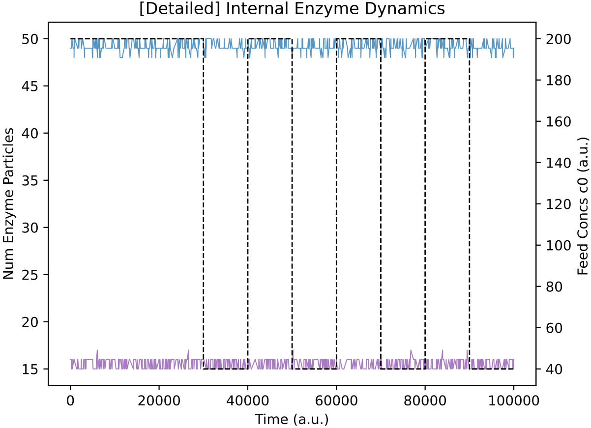
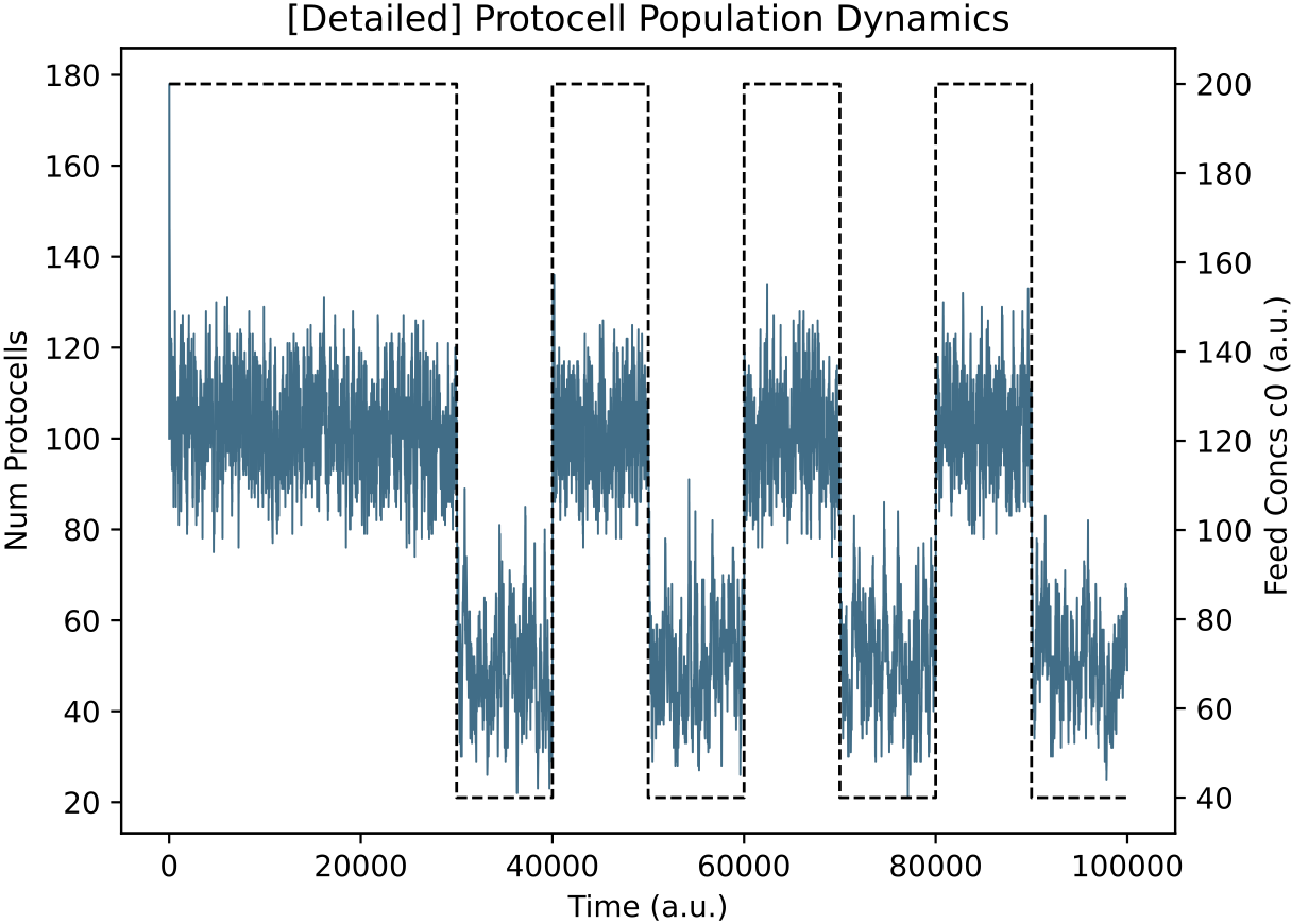
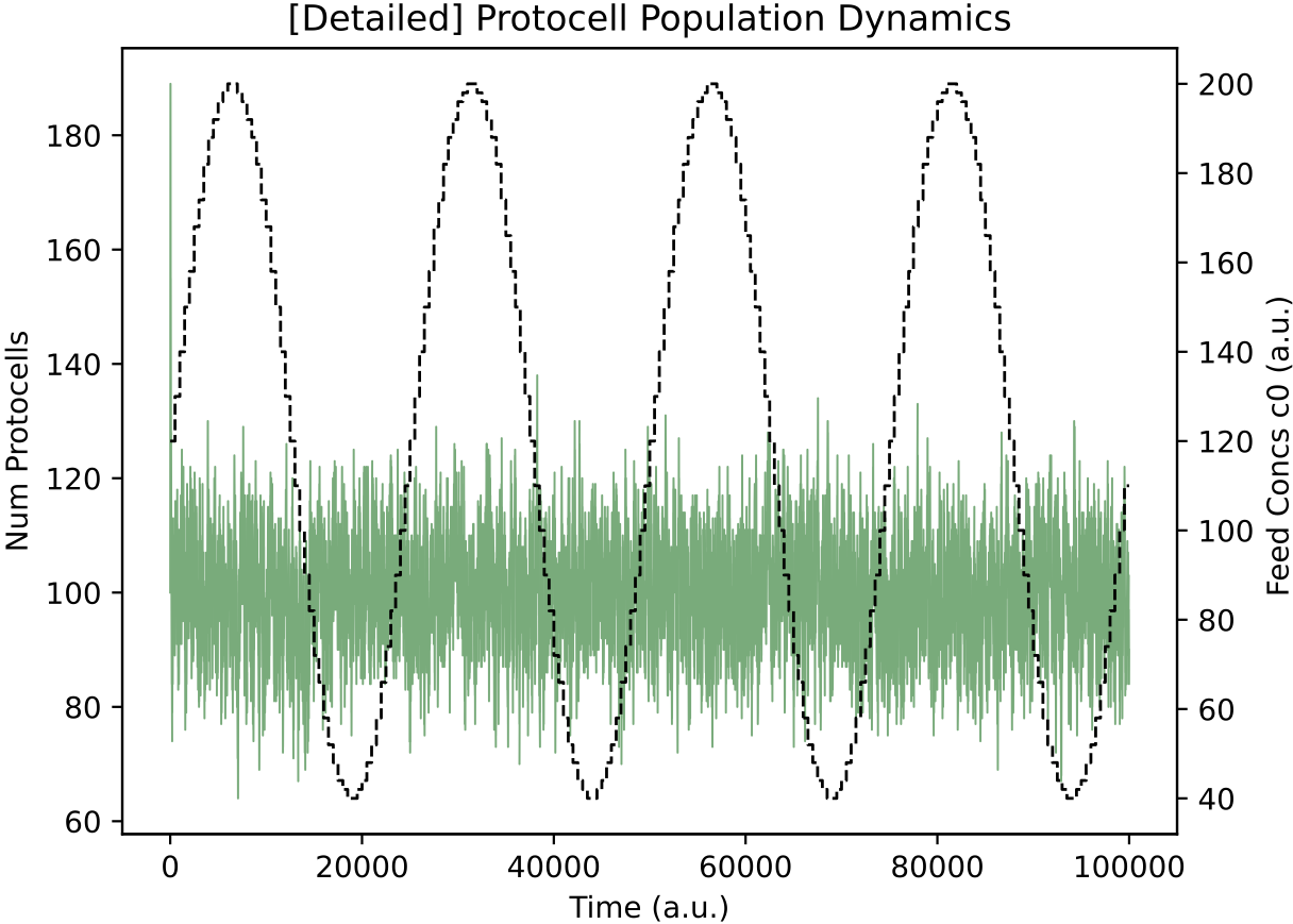
This protocell type is indeed indifferent to external nutrient perturbations (left; E0 = blue, E1 = purple) and its population size oscillates with nutrient availability (right).

For interest, we can also see how the p19055 regulatory network from above behaves when nutrient levels vary as smoother sine waves, rather than as all-or-nothing square waves:

python3 r5b.py
python3 a5.py

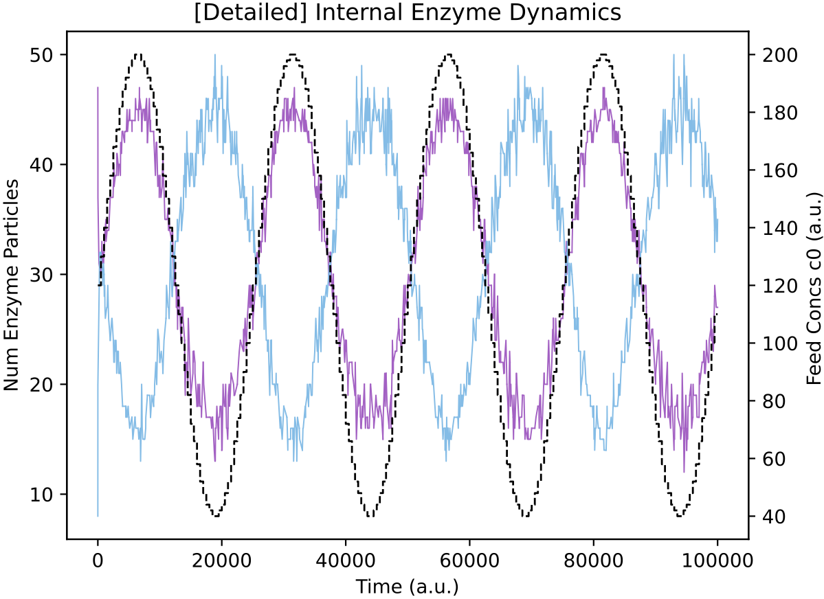
It appears this protocell type has learnt a general relation between nutrient availability and internal enzyme levels: its response is not specifically dependent on nutrient availability varying as a square-wave.

Demo 6: Cross-Feeding Ecology Emerging from Initial Condition

Instead of starting with a single protocell type population, in this demo we start with a very large and heterogeneous population: 50 random protocell types at 100 copies each. The chemostat is supplied with 3 constant nutrient feeds. Evolution and regulation are disabled.

In some cases, a small self-sustaining ecology will emerge from the initial chaos where the members successfully cross-feed from each other:

python3 r6.py
python3 a6.py

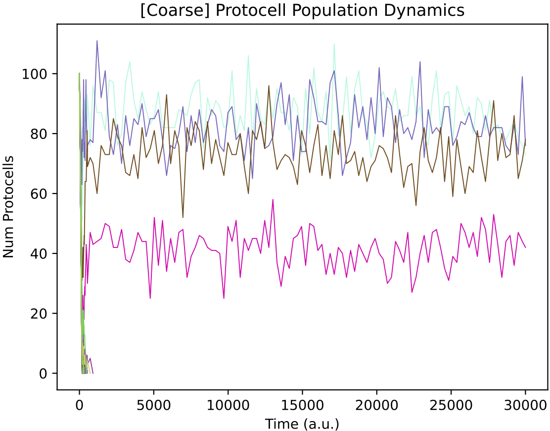
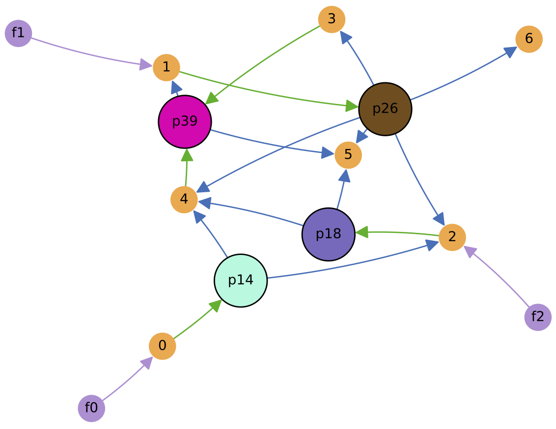
Demo 6: A surviving cross-feeding protocell ecology (trajectories)

Demo 6: An surviving cross-feeding protocell ecology (cross-feeding graph)

In this case, a simple cross-feeding ecology of 4 protocell types emerges from the initial random population: protocell types p14, p26 and p18 feed from single supplied nutrients 0, 1 and 2 respectively, while protocell type p39 cross-feeds from metabolic by-product 4. Also, p39 cross-feeds from metabolic by-product 3 produced by p26.

Note that in the file r6.py that starts the simulation, setting "min_ptypes_to_continue" is set to 3. This means that the simulation will be stopped prematurely if the total number of protocell types in the chemostat drops below 3. Therefore, it could be necessary to run this simulation multiple times in order to observe a self-sustaining community of 3 or more members to 30000 time units.

The total ecological diversity obtainable is dependent on the simulation parameters, the chemical universe, and the particular initial condition. It is worthwhile to highlight that the underlying mathematical model enforces that no ecology can be a ‘perpetual motion machine’ and sustain in the absence of the chemostat nutrient feeds. Each protocell type always imports growth value (as nutrients) at a greater rate than it excretes growth value (as by-products).

Demo 7: Cross-Feeding Ecology under Evolution (Major Innovations Enabled)

In this demo, we take a self-sustaining ecology and go one step further: to see how the population structure changes over a longer evolutionary time.

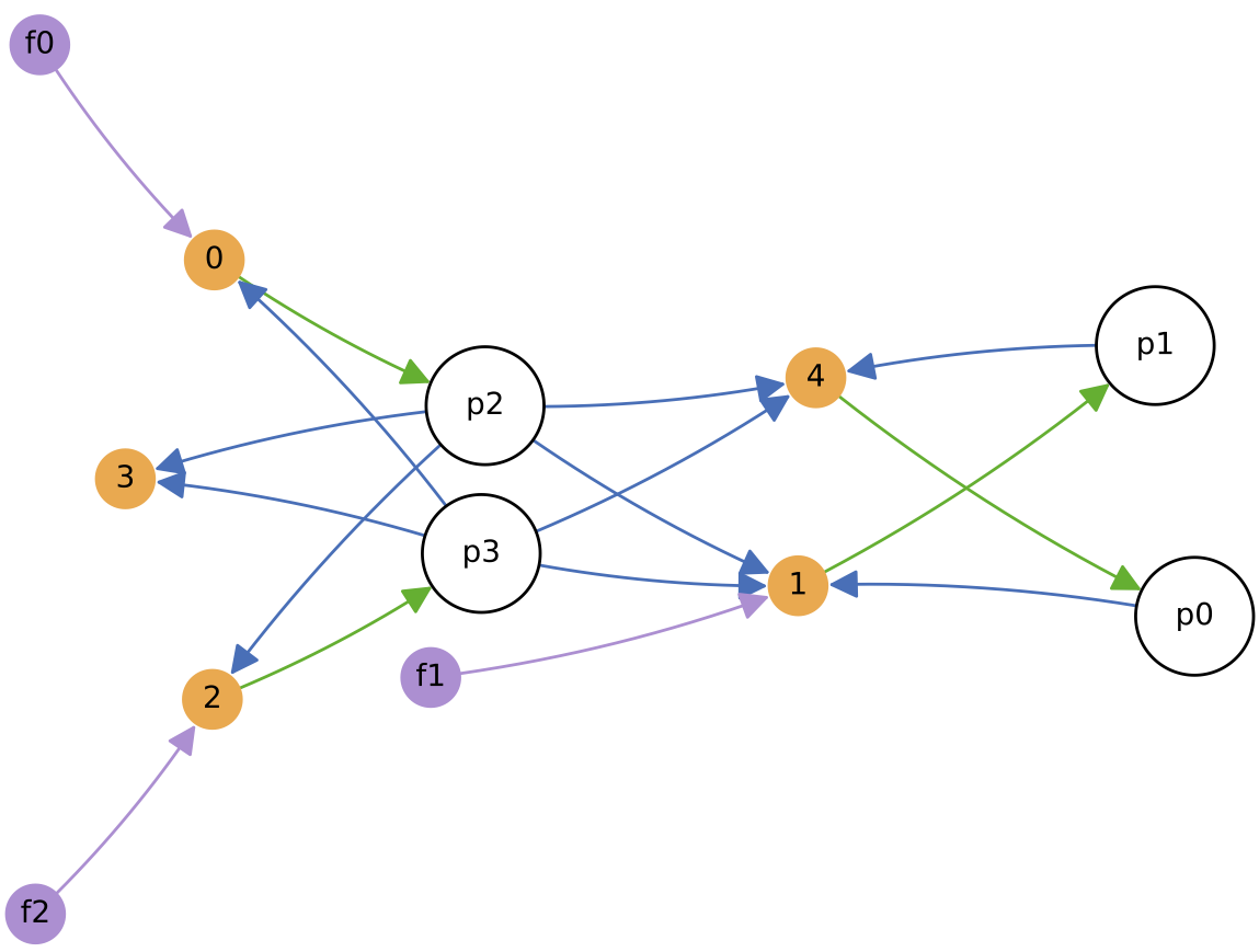
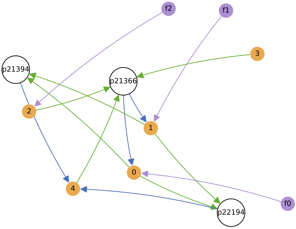
The chemostat is initialised with a self-sustaining ecology of 4 protocell types (shown on the diagram to the right, at 100 copies each), and is fed with three constant nutrient feeds. Evolution is enabled and major innovations are enabled, so protocell types can change both their nutrient ‘diet’ and the number of excreted metabolic by-products over time. Regulation remains disabled.

python3 r7.py
python3 a7.py

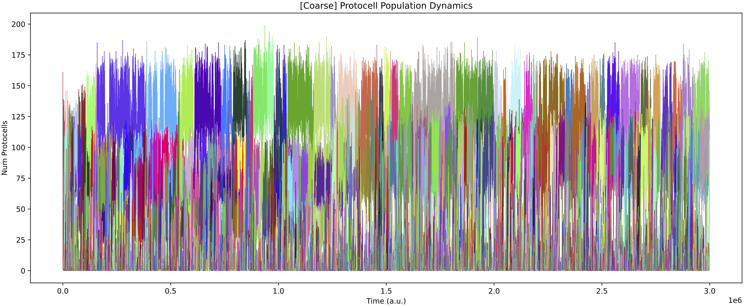
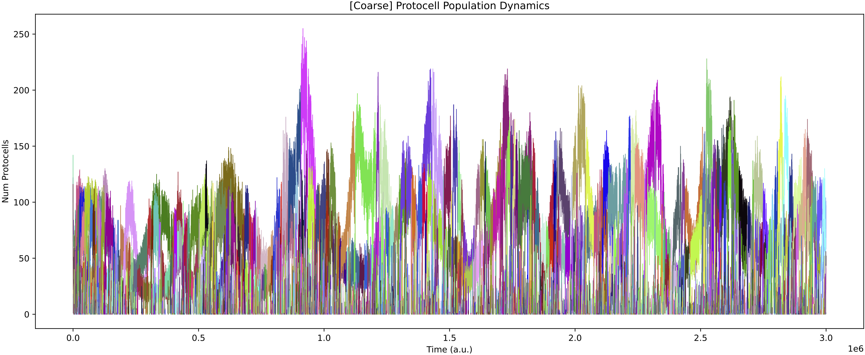
The population structure shifts in non-trivial ways during 3 million time steps:

Changing the "ecology at time t" variable in analysis script a7.py and then re-running this script allows to see the cross-feeding relationships at different time points of the simulation.

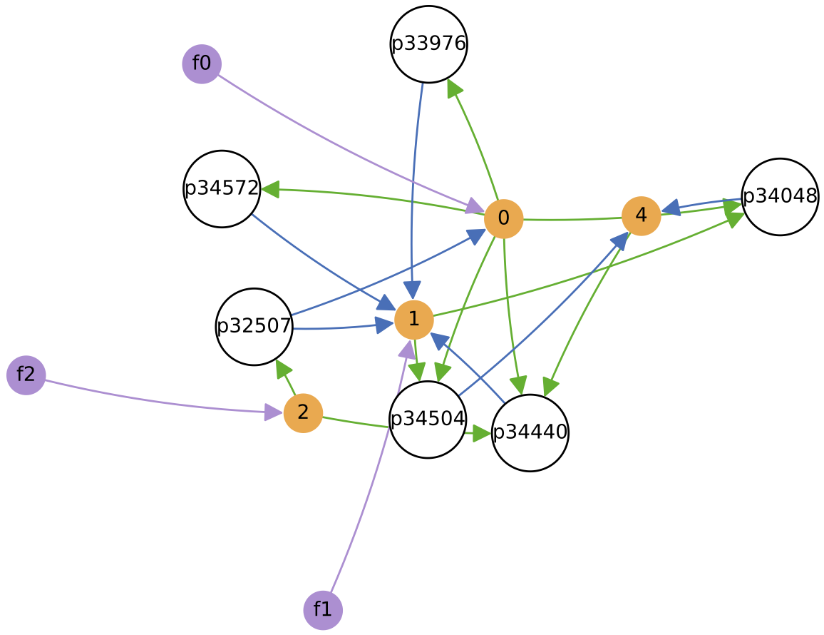
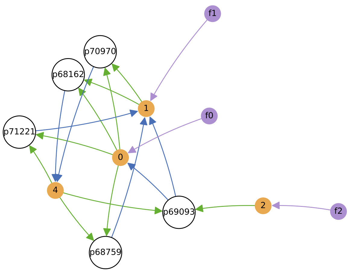
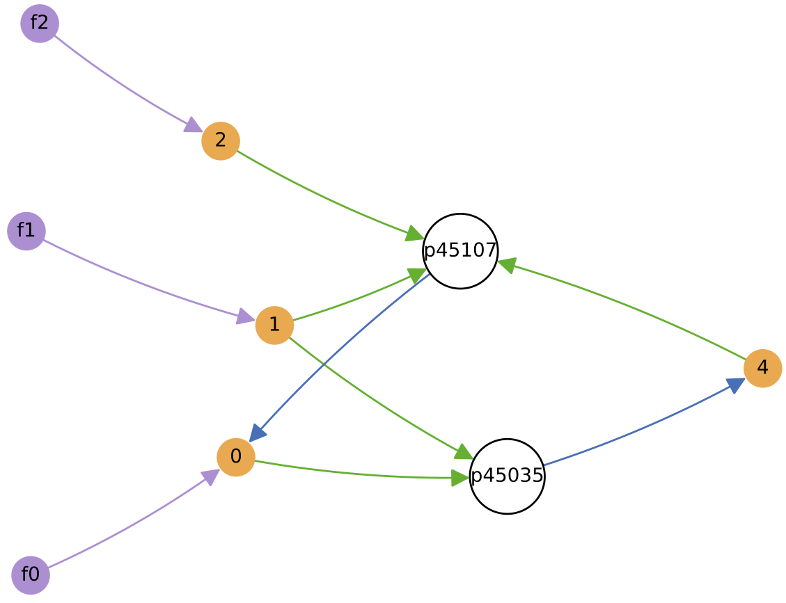
Below shows the ecology at t = 1 million time units, and t = 2 million time units. Because "significant mutants only" is set to True in a7.py, ecology diagrams only include those protocell types that survived long enough to produce a daughter variant (other ephemeral protocell types that may have also existed at the time are not included):

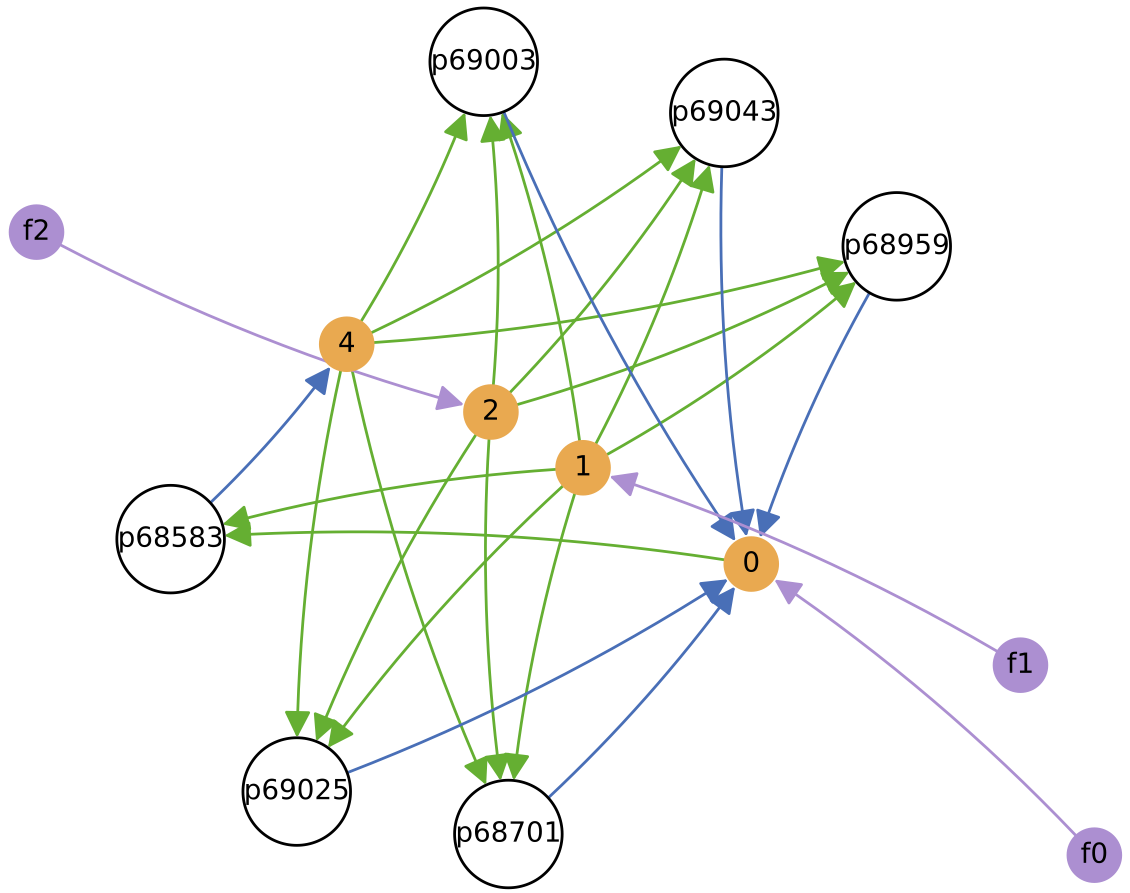
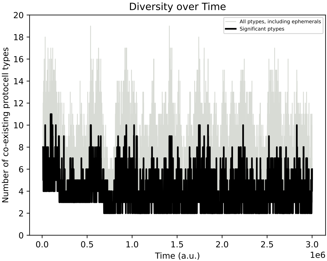
Below shows ecology at t = 3 million time units, and the diversity of protocell types in chemostat over time (mean of around 6 types):

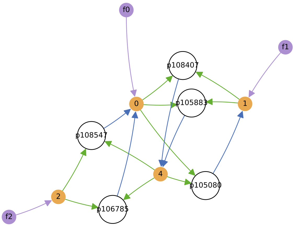
In this particular simulation run, the number of protocell types reduces to 3 core types over time (although “quasi-species” variants can also be present). Each of these core protocell types evolves to have not 1 but 2 nutrient inputs. Thus, the routes of energy/matter flow through the ecology diverge substantially over time from those in the initial ecology above. All protocell types evolve to feed from at least 1 nutrient source directly. Also, protocell types evolve to stop excreting chemical 3 (which is not used in further cross-feeding interactions) fairly quickly.

It is interesting to ask under what conditions can the diversity of protocell types in the ecology actually increase over time. Different initial conditions and nutrient forcing can be expected to produce different evolutionary phenomena.

Demo 8: Cross-Feeding Ecology under Evolution + Varying Nutrient Sources

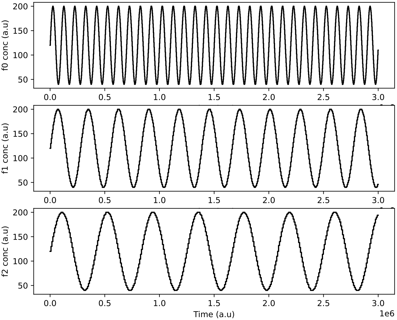
Here, the same initial protocell ecology as in Demo 7 above is used, but this time the nutrient feeds to the reactor are varied as sine waves with different periods (100000, 277000 and 416000 time units, respectively):

python3 r8.py
python3 a8.py

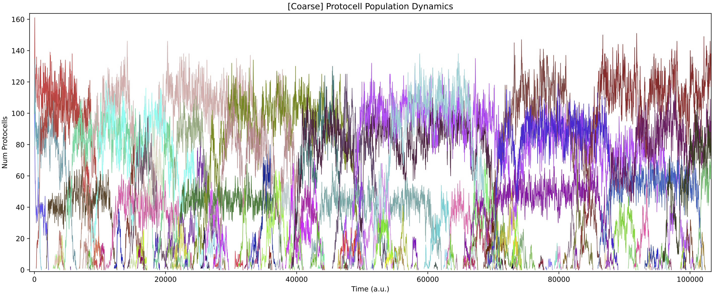
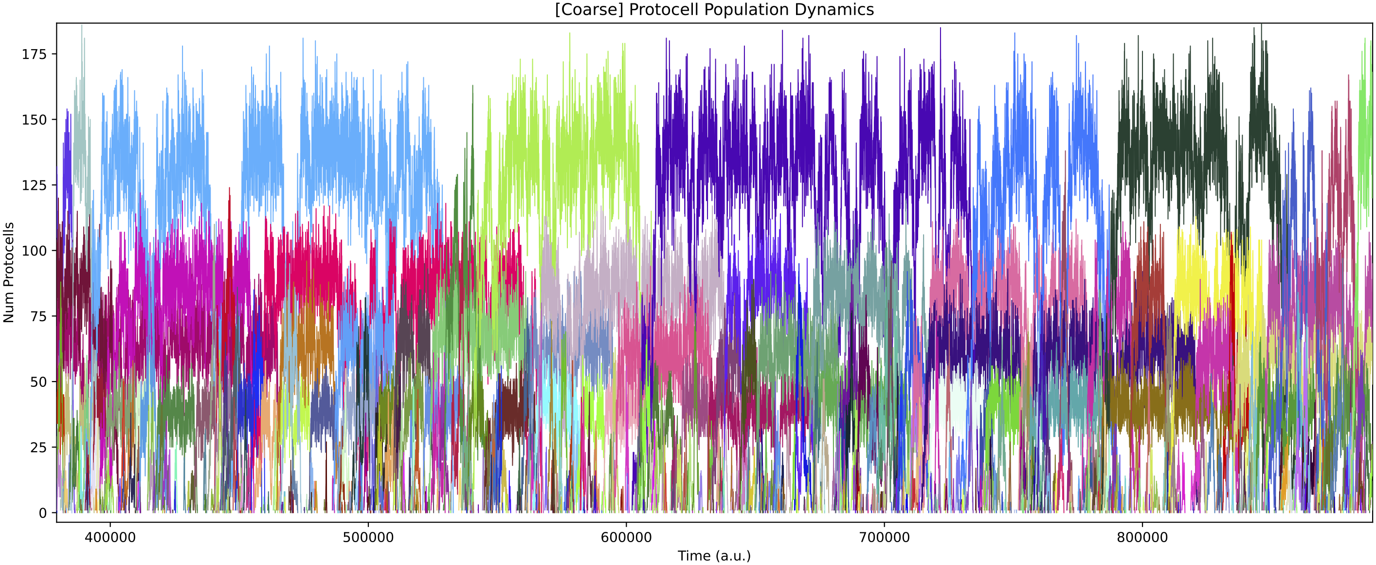
The population dynamics oscillate and partially follow the feed oscillations (depending on the population structure at the time):

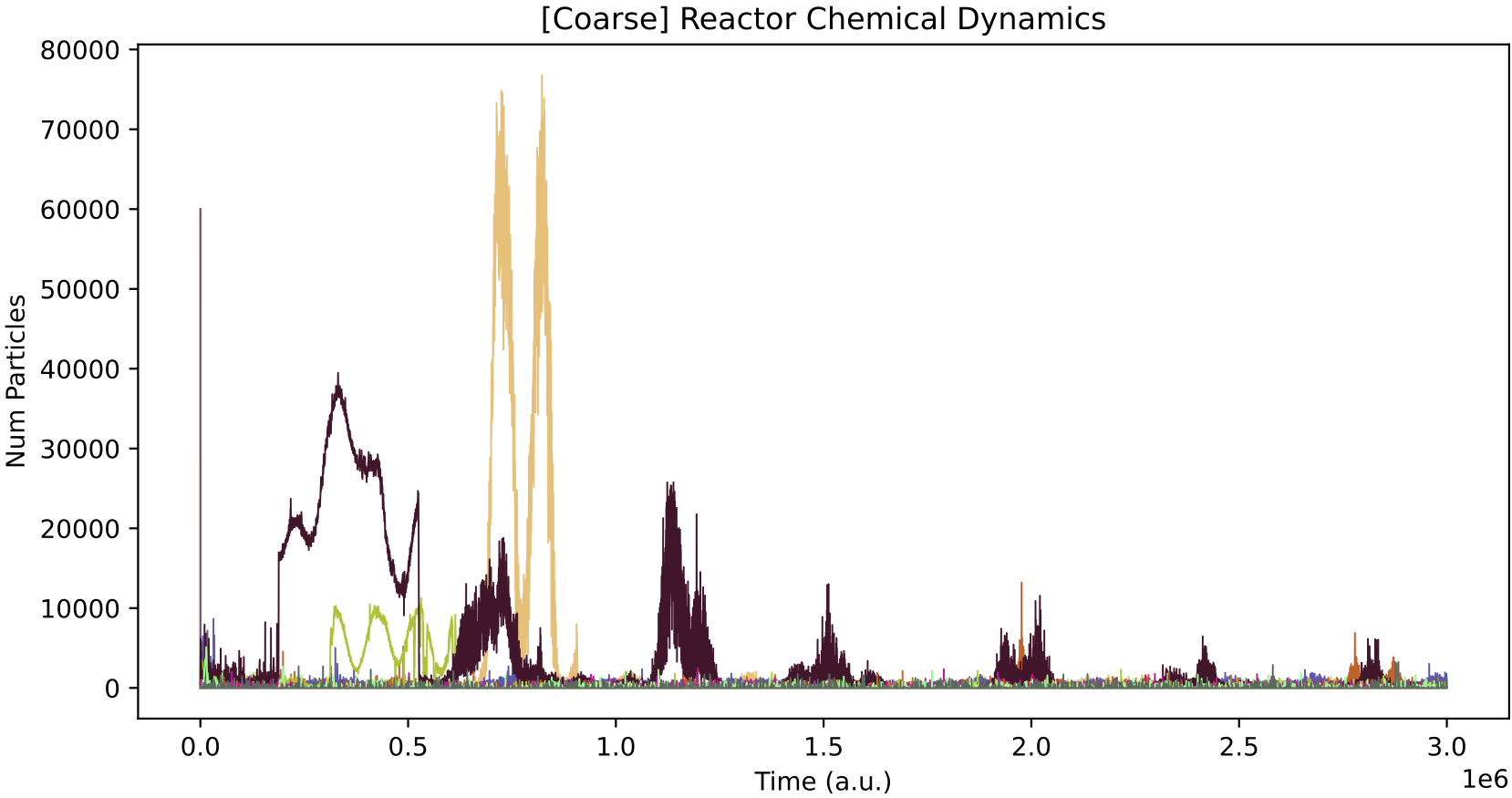
Chemical dynamics in the chemostat also go through distinct phases dependent on how the population structure is shifting:

Below shows the ecology at t = 1 million time units, and t = 2 million time units.

Below shows the ecology at t = 3 million time units, and the diversity of protocell types in chemostat over time:

Finally, the evolutionary lineages for the four initial protocell types (of which, only the descendants of 2 survive):

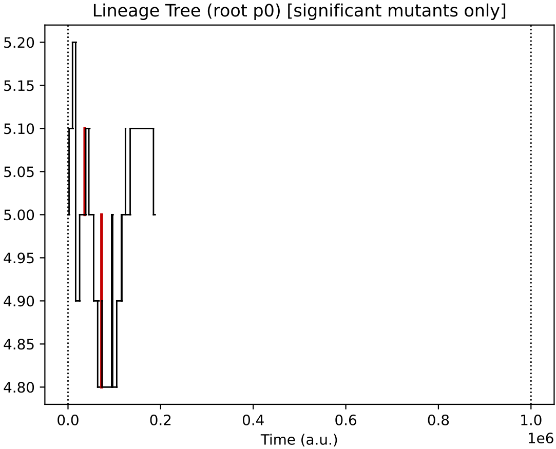
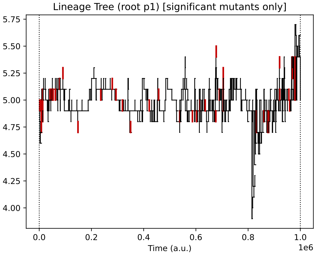
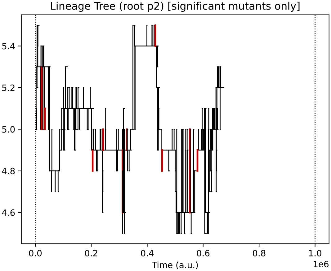
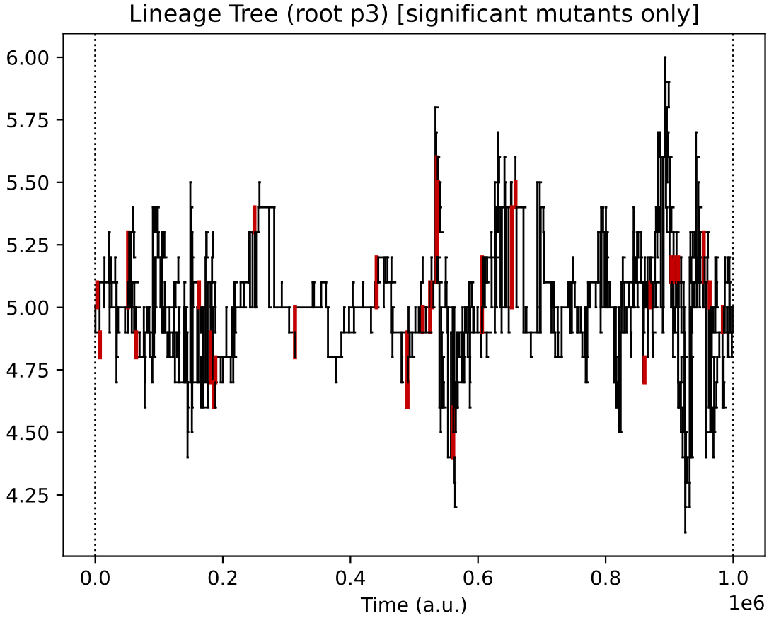
In this particular simulation, under oscillating nutrient forcing, the initial ecology of 4 types reduces to just 2 core types (and their similar quasi-species).

This 2-type arrangement, where one feeds on supplied nutrients 0 and 1, and the other on supplied nutrients 1 and 2 seems to be evolutionary stable in this reactor forcing context.

Demo 9: Cross-Feeding Ecology under Evolution + Varying Nutrient Sources + Regulation

This demo follows the same lines as Demo 8, but now regulation is enabled and protocell species can evolve to vary their internal enzyme levels over short time scales:

python3 r9.py
python3 a9.py

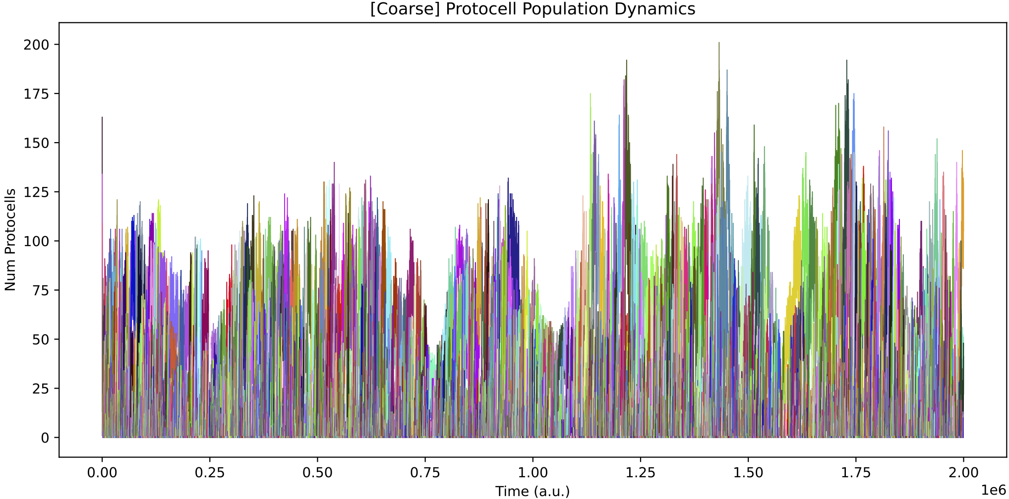
Again, the population sizes vary with the nutrient forcing, but in a less pronounced way than in Demo 8:

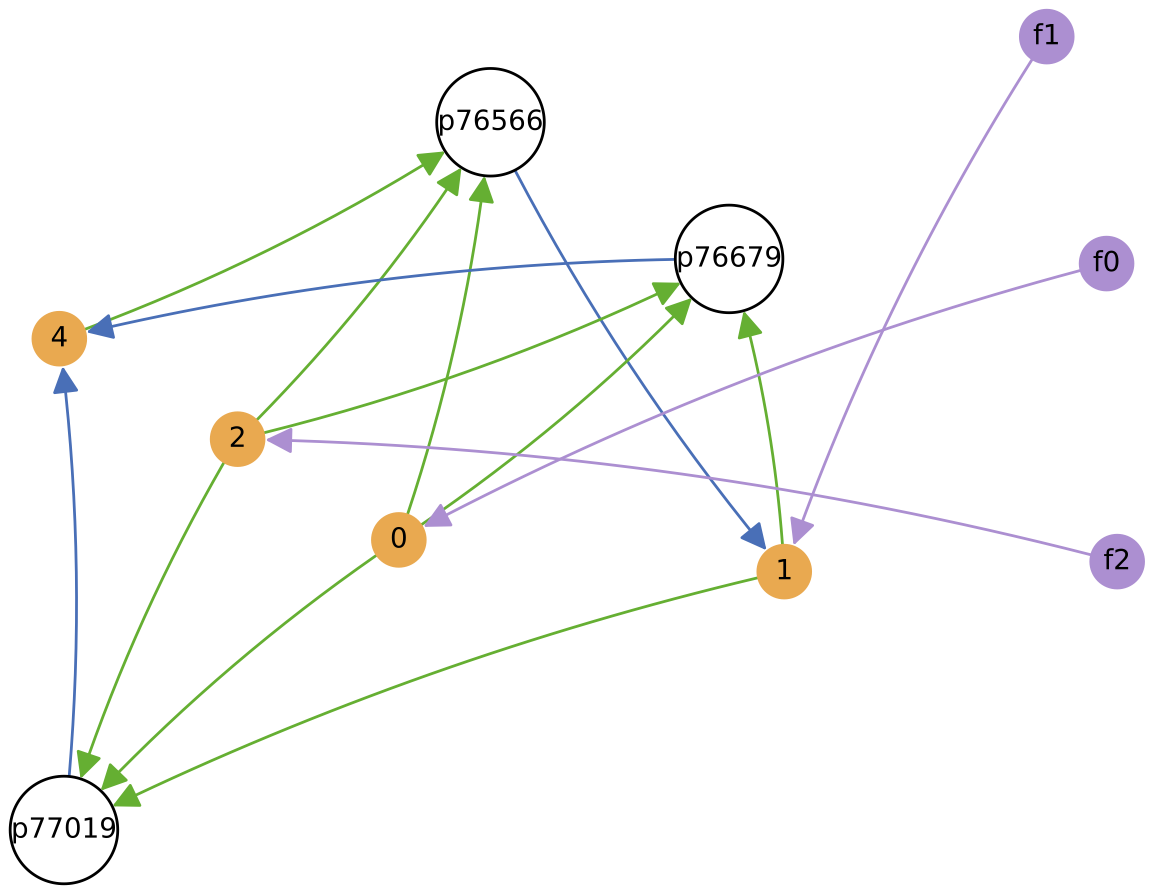
This time, the protocell ecology at the end time (right) has only 2 core species (p76679 and p77019 being related ‘quasi-species’). One species feeds from nutrients 0, 1 and 2, while the other feeds from nutrients 0 and 2. Both weakly cross-feed from each other, also.

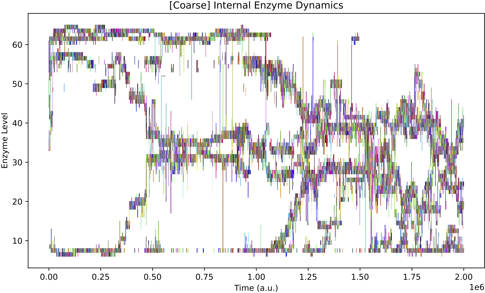
The internal enzyme dynamics of species don’t seem to evolve to track the chemostat nutrient forcing, possibly because the ecological arrangements already buffer this particular scenario of nutrient availability:

However, even if explicit adaptive behaviour may not have evolved in individual protocell species, in this simulation, the population diversity over time involves much more pronounced oscillations as compared to Demo 8:

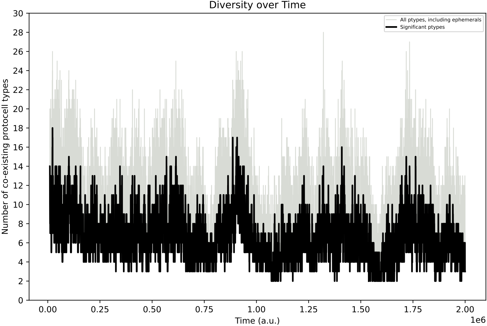
This hints that the inclusion of regulatory capacities (and the longer phenotype associated to each protocell type) can influence evolution in more subtle indirect ways. More investigation of this case, and the response to different nutrient input forcings would be beneficial.

In general, adaptive regulatory capacities do not evolve in all simulations. It is interesting to demarkate under which ecological conditions adaptive regulatory behaviours emerge, and under which they do not. Many different scenarios can be tried with Araudia!

Paper Case Studies

The case studies described in Our Paper can be run by the commands below. Note that in the casestudyX.py files below:

The "regulation_on" flag should be set to False and True for each Case Study, to compare evolutionary trajectories.
The nutrient forcing speed can be selected by setting the reactor_feed_filename variable to the slow, medium or fast forcing CSV filenames.

Case Study 1 - ‘single protocell species’:

cd demo
python3 casestudy1.py
cd ..
cd rstb
python3 analysisB1.py

Case Study 2 - ‘minimal mutualism’:

cd demo
python3 casestudy2.py
cd ..
cd rstb
python3 analysisB23.py

Case Study 3 - ‘binary asymmetric ecology’:

cd demo
python3 casestudy3.py
cd ..
cd rstb
python3 analysisB23.py

The data analysis scripts used above are specific analysis scripts developed for the specific research questions in our paper. They track the “main trunk” protocell lineages, and graph quantities of interest over the lineage.

The above simulations can also have general data analysis performed (like the Demos 1-9 above) by using the araudia/a.py script.

Simulation Challenges

Some practical challenges to keep in mind are:

Simulation speed. When regulation is turned on, neural network calculations are additionally required and simulation speed drops significantly. HPC computing to run repeats becomes necessary.
Data size. Longer simulations require the storage of millions of files, which can amount to several gigabytes of information. Making analysis graphs for very long simulations takes up to 30 minutes, and graphs have a high memory requirement (although specific code optimisations have been performed to mitigate this).
Data analysis complexity. Analysing exact what happens in a population under certain nutrient forcing conditions can require the development of specialist analysis scripts (as was done for Our Paper in the rstb/ directory). Particularly, if the ecology structure is shifting over time due to major evolutionary innovations, this requires more advanced lineage tracking to extract meaningful information about how the population is adapting and cross-interacting over time.